Monte Carlo Simulation

To model a distribution of portfolio results in ClariNet LS, we provide a Monte Carlo simulation model. We calculate survival probability curves for each insured in the same way as the regular Portfolio Valuation model, but we then generate a large number of potential outcomes using the inverse transform sampling method.

Algorithm

Simulation of date of death

The process for generating a simulated date of death for each insured life in the portfolio is as follows:

• Use the LE report(s) for the insured, combined with the specified mortality table to calculate a survival curve (CDF), which will have this form:

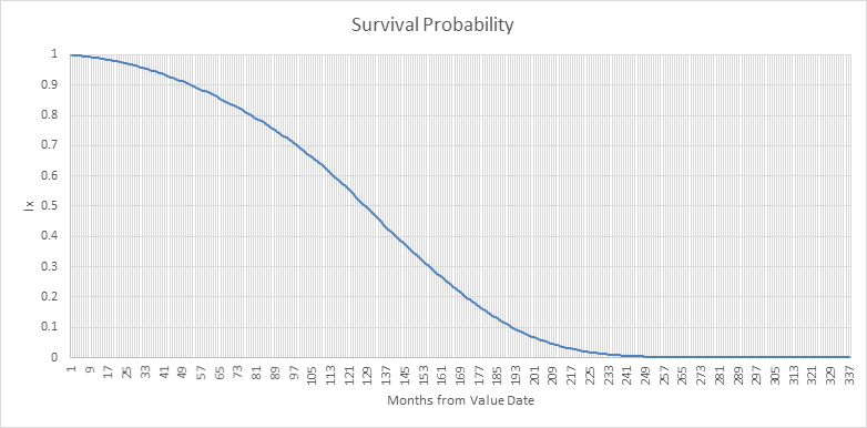
• Generate a set of uniformly distributed, pseudo-random numbers in the range [0,1).
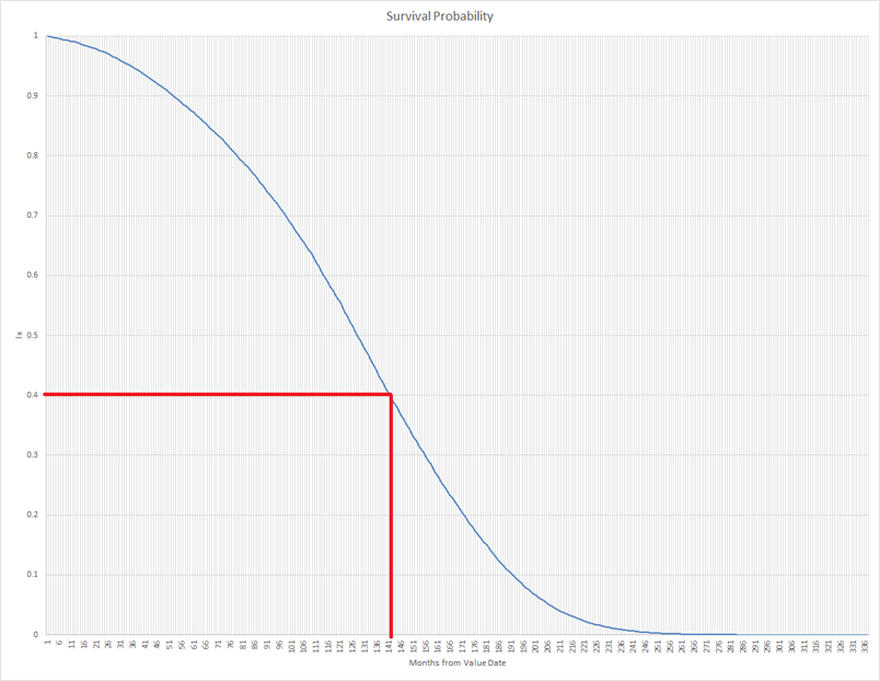
• For each random number, apply this value to a numerical inversion of the survival curve to calculate a date of death for the insured life. Informally, use the random number as the value of the y-axis on the chart above and look where the line meets that point, for example with a random value of 0.4, the date of death is simulated as 141 months from Value Date:

Properties of the simulated date of death

The full details of the survival curve calculation are beyond the scope of this document, but briefly, we are given a mortality table that specifies the mortality rate per year for the insured (qx), starting at the Underwriting Date. We apply a mortality factor to this rate (the MF is generally calculated from the LE50 in the underwriter report and a VBT). We then calculate the survival probability at the end of each month.

The expected future lifetime (mean LE50) is defined as:

$$E(T_X)=\int p_X(t)dt$$

Since our distribution function is discrete, this value can be calculated by summing the survival probabilities in the discrete CDF.

The variance is defined as:

$$V(T_X)=E(T_X^2)-E(T_x)$$

where:

$$E(T_X^2)=2\int t{p}_X(t)dt$$

This can be calculated by summing the survival probabilities in the discrete CDF multiplied by the year fraction from the Value Date at each point on the curve.

Cash flows calculation

Given the date of death for each insured in the portfolio, we can calculate the Net Death Benefit and premium payments for that simulation. We simply assume that if the simulated date of death is before policy maturity, a payment of NDB occurs on the date of death (plus the lag period) and we assume that the projected premium stream is paid from Value Date until the simulated date of death. Given these cashflows, we can generate various policy metrics including a simulated NPV and a simulated IRR (given a Purchase Price).

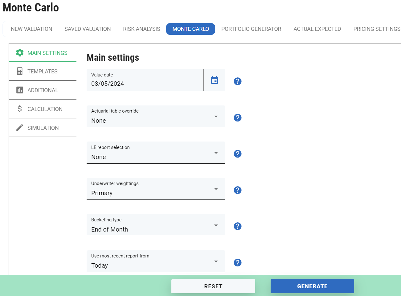
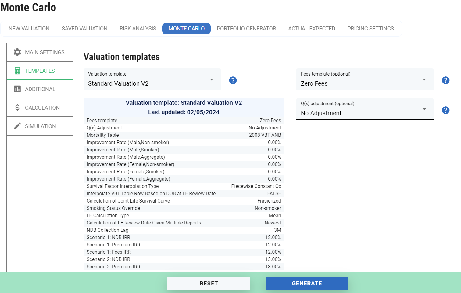
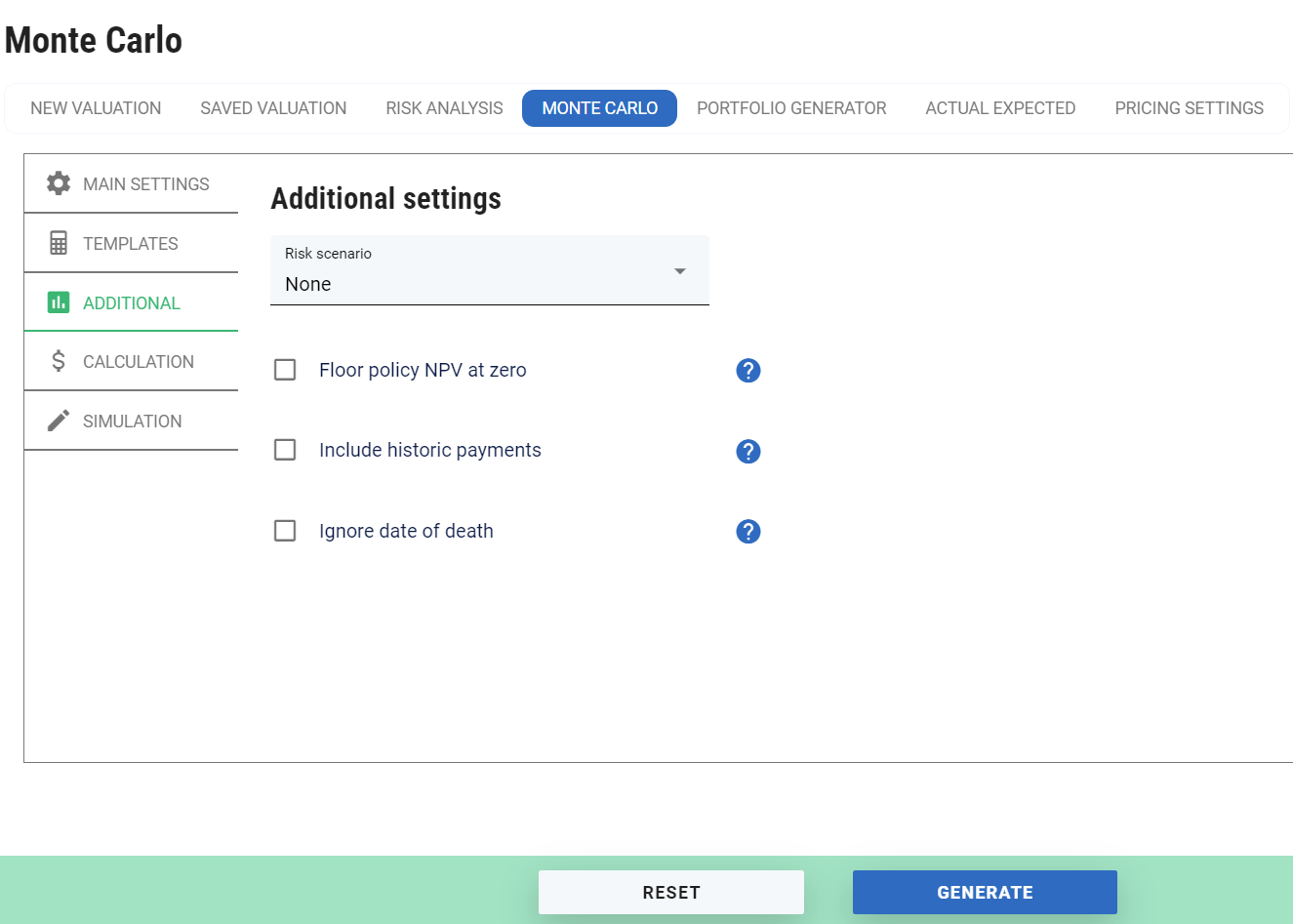
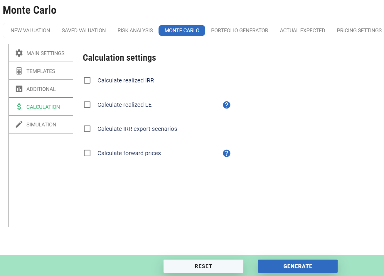
Using the Monte Carlo Simulation screen in ClariNet LS

The Monte Carlo Simulation screen in ClariNet LS looks like this:

Valuation Parameters

These parameters are not specific to Monte Carlo but are used in all policy valuations in ClariNet LS and determine how survival curves are calculated and how cash flows are generated from those curves.

Simulation Parameters

These parameters are specific to Monte Carlo Simulation.

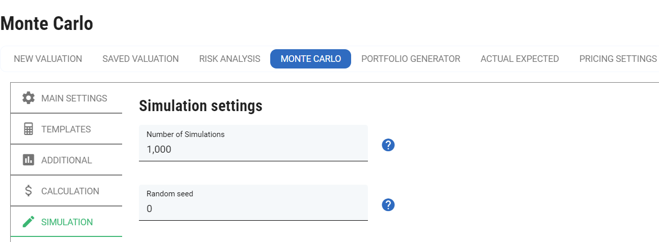
Number of simulations: the number of trials used by Monte Carlo. Note that we use antithetic variables to reduce variance, so the number of unique random numbers will be half the specified number of simulations.

Random seed: a value other than zero is used as a seed by the pseudo-random number generator. If zero is specified, a time-based seed is used, leading to a unique set of results each time.

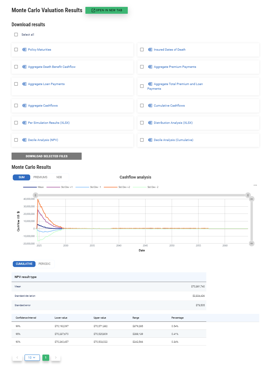
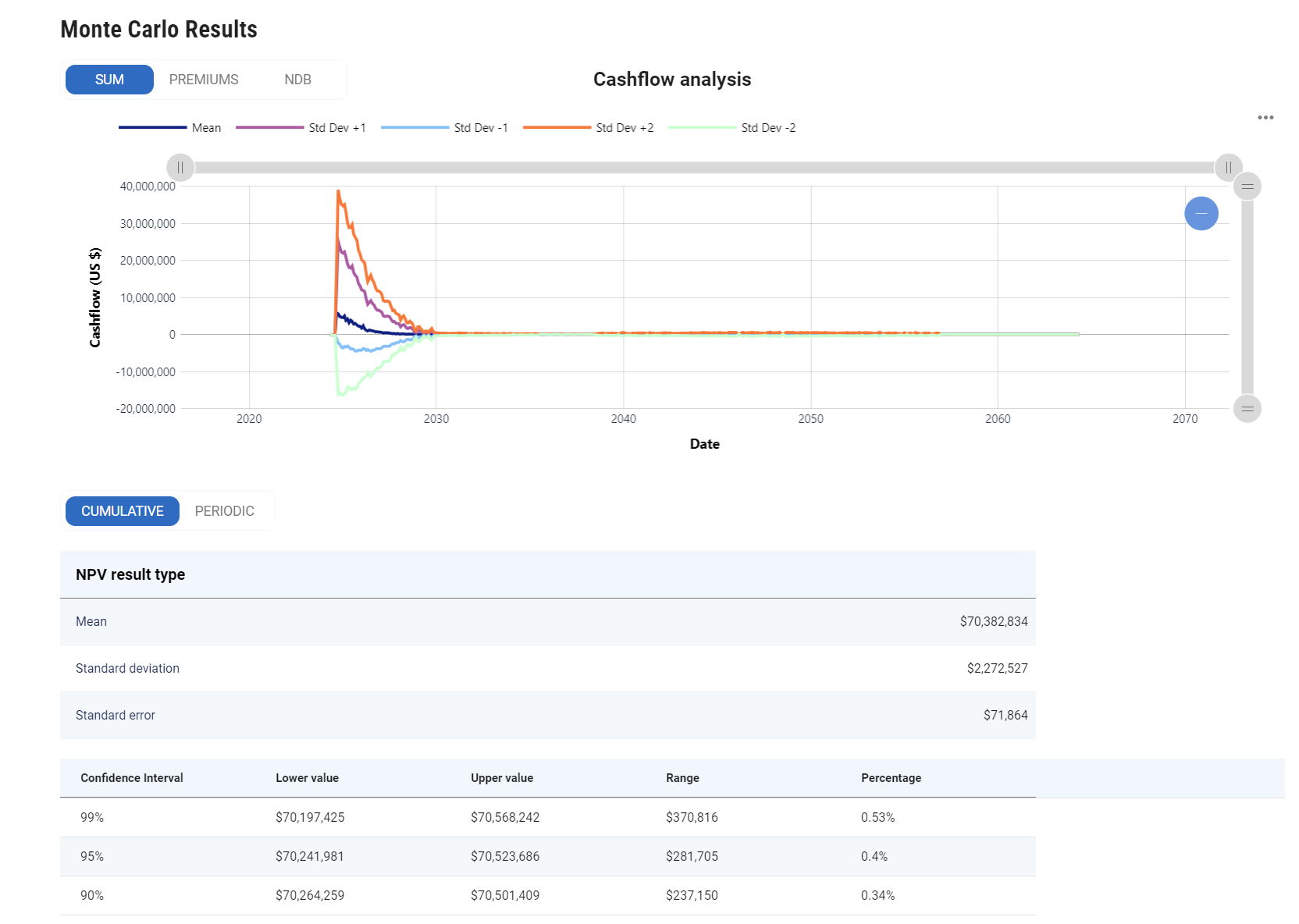
Simulation Results

The first section of the results contains a chart of the mean cash flows resulting from the simulation. Below that we show the NPV statistics. The NPV statistics are useful for comparing the Monte Carlo results to the portfolio valuation results since the former should converge to the latter given a sufficient number of simulations.

Download Results

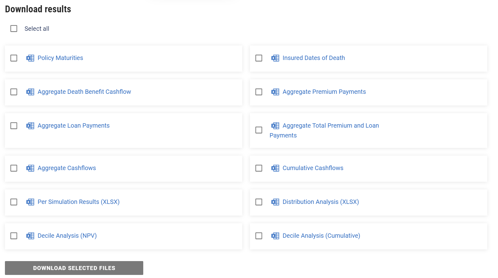
Dates of Death: this CSV gives you access to the maturity date simulated for each policy in each Monte Carlo trial;

Aggregate Cashflows: here you can download the simulated cash flows for the entire portfolio for each trial;

Cumulative Cashflows: this is the aggregate cash flows, but on a cumulative basis over time;

Per Simulation Results: This file contains the NPV, NDB NPV, Premium NPV, Realized IRR, Unweighted Realized LE50 and Weighted Realized LE50.

Distribution Analysis: this sheet contains simulated cash flow results with various percentiles, for risk analysis.

Decile Analysis: another form of cash flow results with percentile analysis.