Interpolation of Mortality Curves

Overview

The ClearLife pricing model has been extended to support piecewise linear interpolation of both the mortality rate $q_{x}$ and the force of death (λ). This means that as one moves between underwriting date anniversaries, rather than seeing a jump in the respective rate, it gradually increases. This parameter is controlled via the Valuation Template in ClariNet (Survival Factor Interpolation Type). The options are:

Interpolation Type	Meaning
Piecewise Constant Qx	q_x constant between underwriting dates.
Piecewise Constant Force Of Death	λ constant between underwriting dates.
Piecewise Linear Qx	q_x linearly interpolated between u/w dates.
Piecewise Linear Force Of Death	λ linearly interpolated between u/w dates.

The Specification of Mortality

For the purposes of this document, we assume that underwriters supply either:

the survival curve

l_{x} (t) for t = 0. . N at annual intervals

or the mortality curve

q_{x} (t) for t = 0. . N at annual intervals

In the case of the survival curve, we will back out the mortality curve using:

q_{x} (t - 1) = 1 - \frac{l_{x} (t)}{l_{x} (t - 1)} where l_{x} (0) = 1

Interpolation

Given that we have $q_{x} (t)$ for each year starting at $t = 0$ (Underwriting Date), we need an estimate for $q_{x} (t^{'})$ where $t^{'}$ is not an anniversary of the underwriting date.

Underwriter	t=0	t=1	t=2	t=3	t=4
Date	2-sep-2011	2-sep-2012	2-sep-2013	2-sep-2014	2-sep-2015
q x (t)	25/1000	50/1000	75/1000	100/1000	125/1000

Given $q_{x} (t)$ and $q_{x} (t)$ , we need a value for $q_{x} (t + t^{'})$ where $0 < t^{'} < 1$ . $t^{'}$ is expressed as a fraction of a year.

We show the four common approaches:

Piecewise constant $q_{x}$ ;
Piecewise linear interpolation of $q_{x}$ ;
Piecewise constant exponential interpolation of hazard rate (λ);
Piecewise linear exponential interpolation of hazard rate (λ);

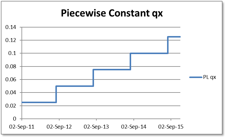
Piecewise Constant Interpolation of qx

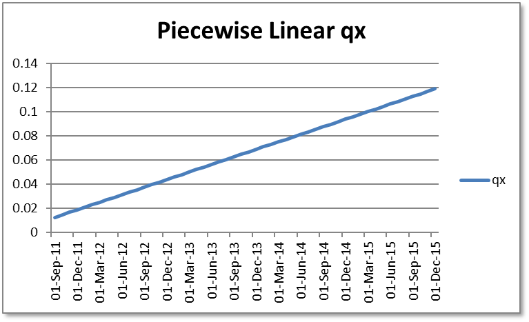
With this approach, we simply assume that $q_{x} (t + t^{'}) where 0 < t^{'} < 1$ . This leads to an interpolation as follows.

Piecewise Linear Interpolation of qx

In the case of piecewise linear interpolation of $q_{x}$ , we calculate an interpolated value of $q_{x}$ between each underwriting date and a slope between each of these interpolated points. This process is straightforward with the exception of obtaining the first interpolated point, which occurs six months before the underwriting date. In order to calculate this, we simply extrapolate backwards using the slope between $q_{x}$ at underwriting date and $q_{x}$ one year later. The calculation is:

The resulting graph is:

q_{x} (2-sep-2011) = q x (2-sep-2011) - [q x (2-sep-2012) - q x (2-sep-2011)] / 2

To contrast the two calculations, the following graph shows them together:

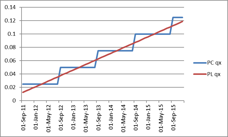
From the graph, it can be seen that in the piecewise linear version, during the first half of an underwriting year, the value is below the piecewise constant value and in the second half of the year it is above. So on 2-sep-2011, PC $q_{x}$ = 0.025, whereas, PL $q_{x}$ = 0.0125. On 2-mar-2012, they are equal.

Exponential Interpolation of Hazard Rate (PC and PL)

The exponential hazard rate model assumes that within each year, mortality events are independent, continuous and occur at a constant rate. For each given value of qx(t), a survival probability is calculated; $p_{x} (t) = 1 - q_{x} (t)$ . Within each year, survival rates are calculated as

Since t=1, the value of λ is calculated as

This gives a table like this:

Date	q x	p x	λ
2-sep-2011	0.025	0.975	0.025318
2-sep-2012	0.05	0.95	0.051293
2-sep-2013	0.075	0.925	0.077962
2-sep-2014	0.1	0.9	0.105361
2-sep-2015	0.125	0.875	0.133531

The interpolation method for piecewise linear λ uses the same approach as $q_{x}$ but using a different rate.